Ψ-Diophantine Lattice
🧮 How to Read the Ψ-Diophantine Lattice
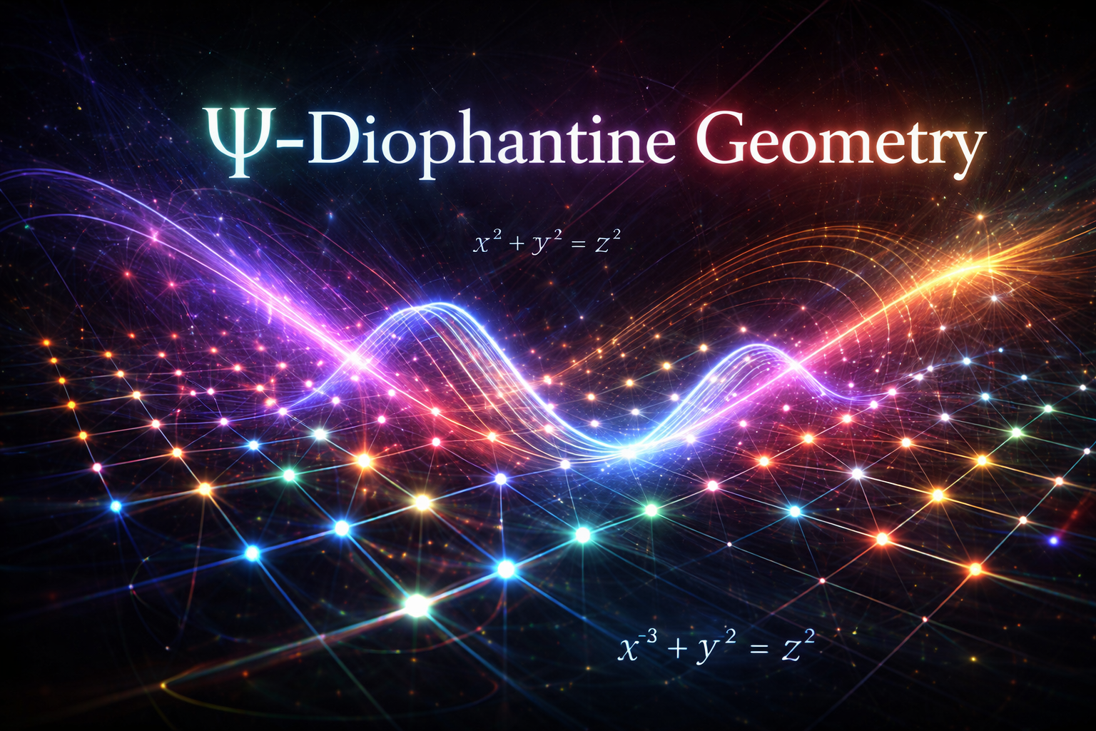
This module visualizes Diophantine equations as geometry — not as formulas to solve, but as constraints shaping integer space.
What you’re seeing
Each point represents an integer pair (x, y). The equation defines a surface these points attempt to lie on.
Bright points satisfy the equation exactly. Faded points miss by a small error. Large gaps reveal structural impossibility.
Why presets matter
Each preset isolates a different mathematical regime:
- Pythagorean — harmonic closure and symmetry
- Cubic — unstable recursion, no closure
- Mixed powers — entropy boundaries
- Quartic — symmetry restoring modular alignment
What this teaches
Solvability is not about luck or numerology — it emerges from geometry, symmetry, and constraint density.
Ψ-Diophantine Lab
Equation Playground
🌀 How to Interpret the Ψ-Diophantine Resonance Lab
This lab does not attempt to solve Diophantine equations directly. Instead, it visualizes the structural character of an equation — how constraint, symmetry, and degree interact.
What the wave represents
The animated curve encodes a resonance profile derived from:
degree number of variables curvature pressure entropy leakage
Equations with strong internal symmetry produce smooth, bounded oscillations. Others fracture into unstable or incoherent motion.
Why presets matter
Each Ψ-preset isolates a canonical regime:
- Ψ-D.1 — harmonic closure (Pythagorean-type)
- Ψ-D.2 — recursive instability (cubic growth)
- Ψ-D.3 — partial solvability under mixed powers
- Ψ-D.4 — symmetry restoration via even-degree balance
How to read the metrics
The reported values are comparative indicators, not exact invariants:
Curvature measures constraint tightness Entropy estimates solution dispersion Resonance reflects structural coherence
This lab is about seeing that difference.
Harmonic Constraint Field
✦ What You’re Seeing — A Harmonic Constraint Field
This animation is not particle noise or random motion. It visualizes a field of constrained degrees of freedom.
Structure first
Each node orbits a shared center, but its motion is limited by: radius phase angular speed
The black lines define the structural skeleton. White outlines reveal orientation without overpowering form.
Why it moves slowly
Slowness makes constraint visible. Fast motion hides structure; slow motion exposes it.
Color meaning
Aquamarine — flow & continuity Jade — stability & constraint Topaz — transition & tension